
Elliptic curves are a class of algebraic curves frequently used in cryptography, most notably in the elliptic curve digital signature algorithm (ECDSA) and some SNARK-based zero-knowledge proofs (ZKPs) such as PLONK. But what are they, how do they work, and why are they used?
This article provides a technical exploration of elliptic curves, their mathematical structure, properties, elliptic curve point addition, and their application in cryptography and ZKPs.
Note that this resource is intended for programmers to familiarize themselves with the mathematical prerequisites for understanding cryptography and zero-knowledge proofs. The mathematical derivations have been omitted for brevity, but resources will be linked for those wanting to understand further.
Elliptic curves are a class of algebraic curve with an equation of the form:
$$y^2 = x^3 + ax + b$$
where $a$ and $b$ are constant coefficients. The curves must be defined over a field $K$, meaning the coordinates $(x,y)$ and coefficients $(a,b)$ must all be elements of field $K$.
This is the most common form of elliptic curve equation, known as the affine Weierstrass form. Others include the twisted Edwards form and the Montgomery form, which will not be covered in this article.
In Figure 1 below, you can see the elliptic curve defined over the field of real numbers, where $a=-1$ and $b=1$
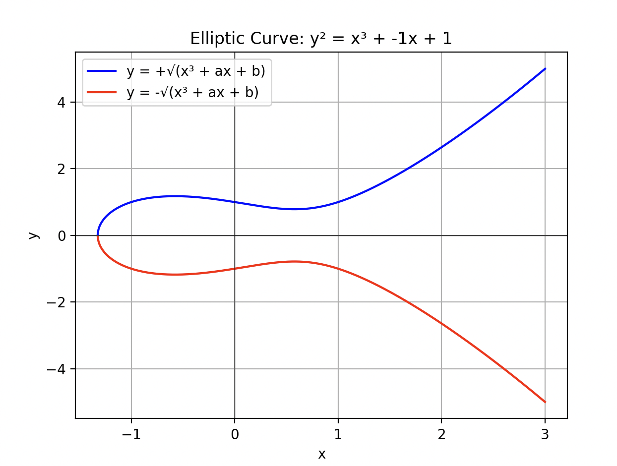
A point $(x, y)$ on an elliptic curve is the value of $y$ and $x$ that satisfies the above equation for a given $a$ and $b$.
The curve must be non-singular (i.e., it has no sharp points, known as cusps, or self-intersections). This is checked using the discriminant $\Delta = 4a^3 + 27b^2$ which must not be zero ($\Delta \not= 0$). This ensures that mathematical operations such as point addition (covered later in this article) are well-defined at every point on the curve.
Elliptic curves must be defined over a field $K$, meaning the coordinates $(x,y)$ and the curve parameters $a$ and $b$ must all be elements of field $K$.
When we refer to elliptic curves "over" some field, we're specifying the set from which all values are drawn:
The elliptic curves we've examined so far have been over the real numbers, which is why Figure 1 shows a continuous, smooth plot. This will be the focus of this article, but note that the same characteristics hold for elliptic curves over finite fields.
The points on an elliptic curve form a set. When considering real numbers, this is, of course, an infinite set of points that satisfy the equation of an elliptic curve. We can also “add” these points together using a binary operator called elliptic curve point addition.
The process of adding together points is a little more complicated than simply “summing the x coordinates and then the y coordinates.” We shall discuss specifically how point addition actually works shortly. Still, the most important takeaway is:
The set of elliptic curve points equipped with the point addition binary operator forms an Abelian group.
And given this fact, we can define this “point addition” operator such that it adheres to the required rules of Abelian groups.
Recall that to be an Abelian group, the set of elliptic curve points under the point addition operator needs to satisfy the following properties (remember the mnemonic Clearly Cyfrin Is Incredibly Awesome):
Where, $P$, $Q$ and $R$ are all points on the elliptic curve with $x$ and $y$ coordinates and $+$ is the point addition operator (not regular addition).
But we still don’t know what this mystical “point addition” operator is so let’s define it .
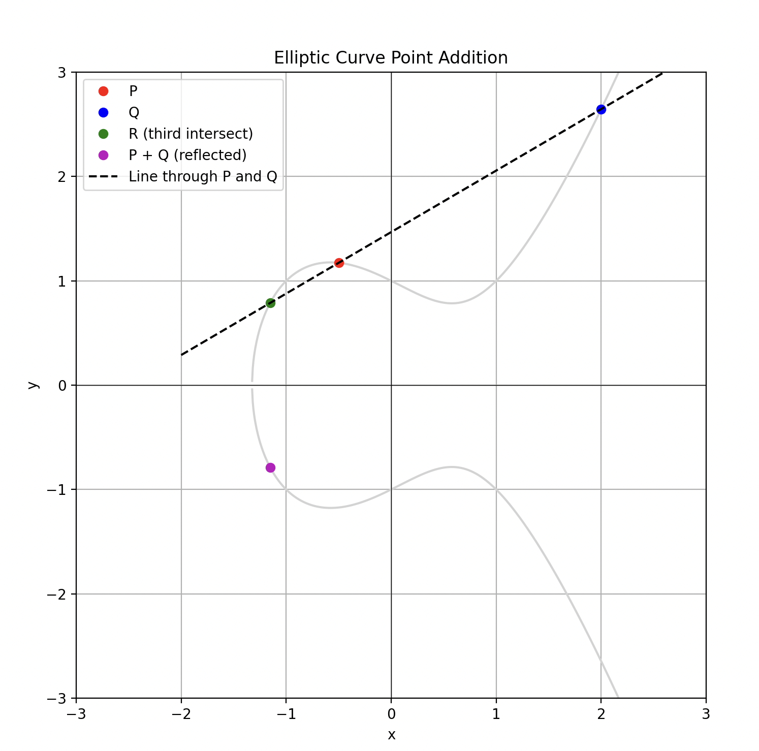
Point addition is the addition of two points $P = (x_1, y_1)$ and $Q = (x_2, y_2)$ on the elliptic curve. It is not addition in the “usual” sense, but instead is defined by the following geometric rules:
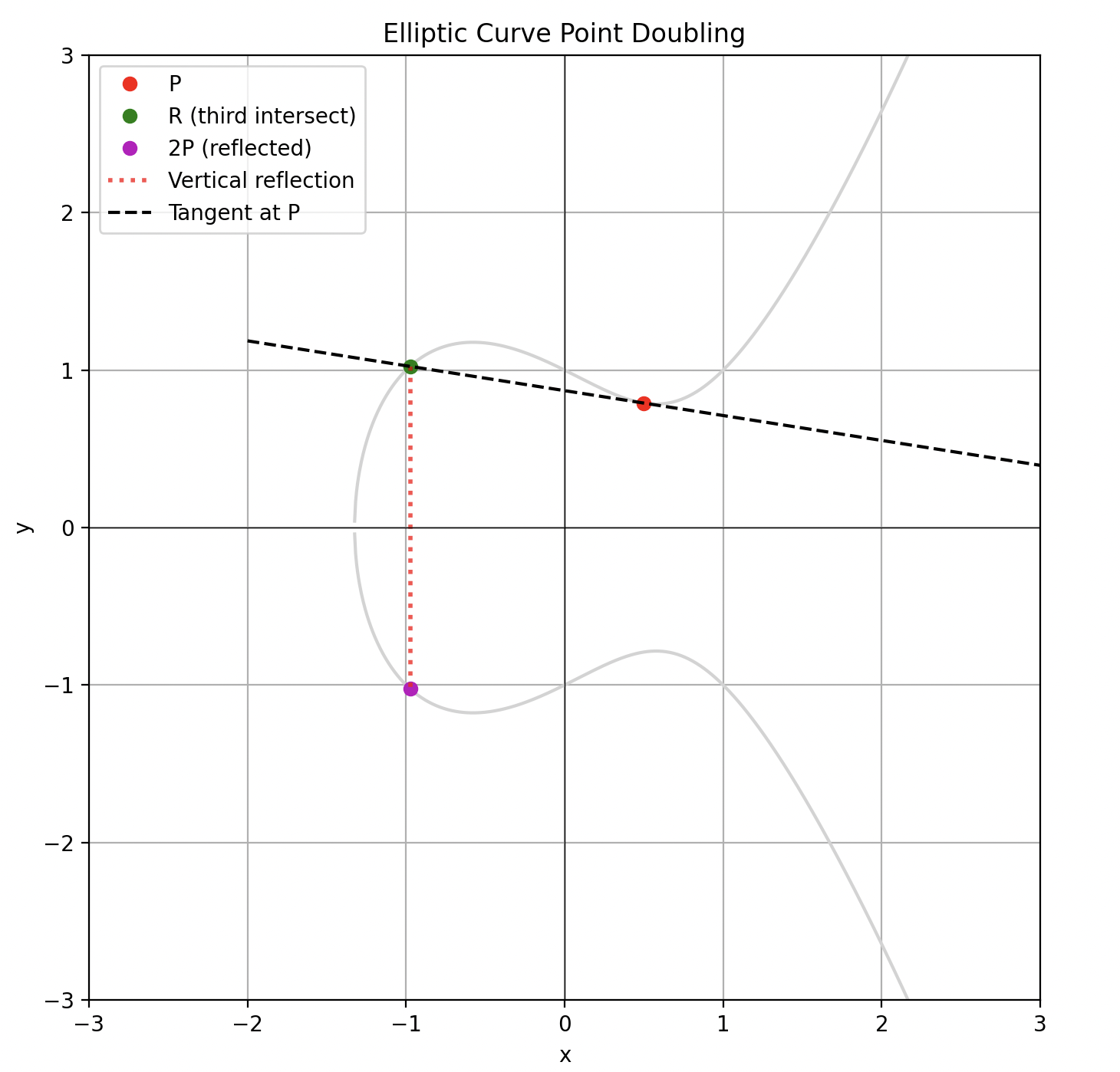
We can use this point doubling to define scalar multiplication of elliptic curve points.
Point multiplication (multiplication between points) does not exist in the group since it is defined with the point addition operator. However, we can use scalar multiplication, which is defined as simply adding a point to itself a number of times equal to the scalar. "Scalar" refers to a regular number (like an integer), rather than another group element. For example, let’s do some scalar multiplication of $P$:
$$2P = P + P$$
$$4P = P + P + P + P$$
Or, more generally:
$$xP = \underbrace{P + P + ... + P}_{ x \space times}$$
This is scalar multiplication! Remember that $+$ is point addition that follows the geometric rules rather than regular addition.
As we’ve said, if you draw a line through two points $P$ and $Q$ on an elliptic curve, it intersects the curve at a third point, call it $R'$.
The key geometric fact is: three collinear points on the curve sum to zero:
$$P + Q + R' = \mathcal{O}$$
Now, suppose we defined addition as $P+Q=R'$. Then this relation would read:
$$P + Q + (P+Q) = \mathcal{O}$$
Which simplifies to
$$2(P+Q) = \mathcal{O}$$
That would mean every sum is its own inverse. This clearly breaks the group laws: we would not have a consistent identity or inverses.
To fix this, we redefine the sum to be the reflection of the third point:
$$P+Q=−R'$$
Now the relation becomes:
$$P + Q + (- (P+Q)) = \mathcal{O}$$
which is consistent with the requirement that every point has an inverse and that the point at infinity $\mathcal{O}$ acts as the identity.
With this definition:
By convention, we write $P+Q=R$, where $R$ is already included with this reflection step.
Let’s now define what $\mathcal{O}$ is.
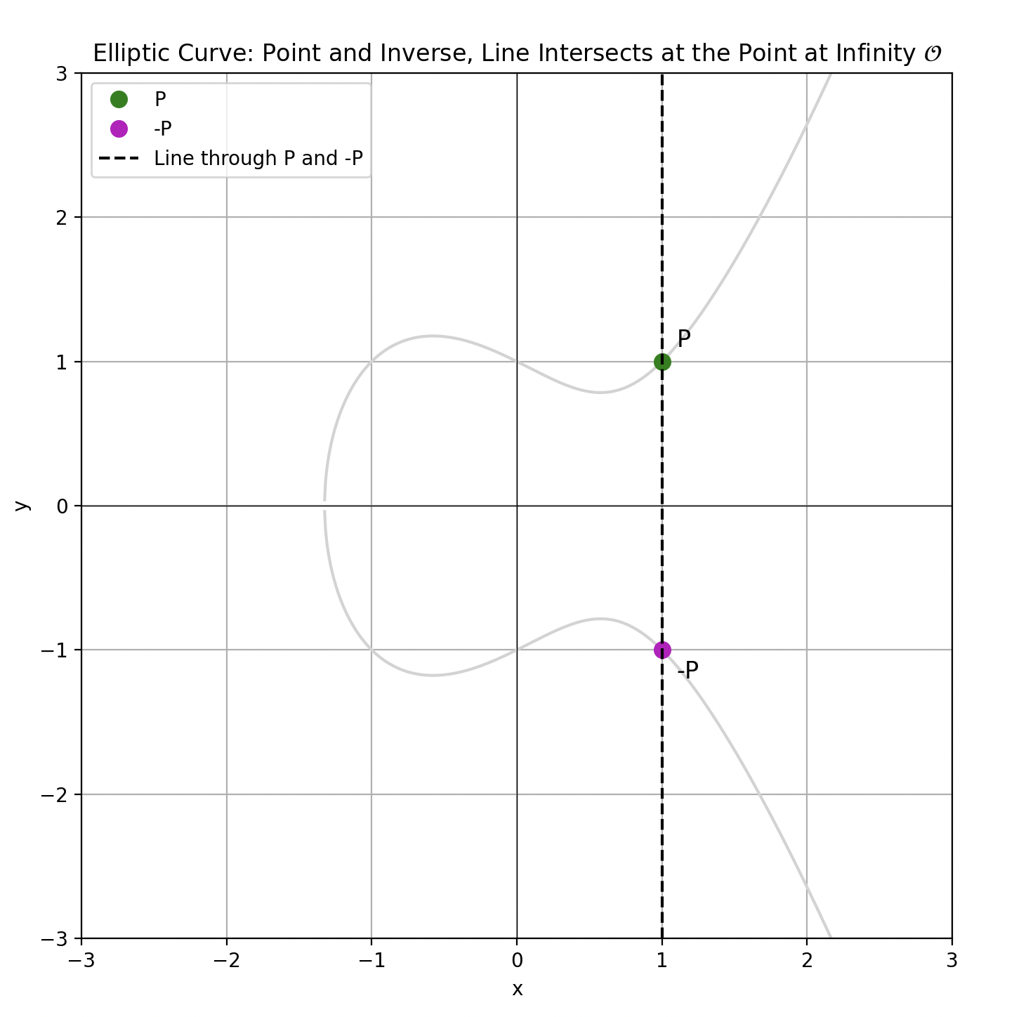
The point at infinity $\mathcal{O}$ serves as the identity element for elliptic curves, such that $P + \mathcal{O} = P$ for all $P$. This is the point at which two parallel lines would eventually intersect.
Intuitively, it may seem logical to say that $(0,0)$ would be the identity element since any point plus $(0,0)$ should return the original point, right? However, this is not the case, which may sound confusing, but here’s why:
Under point addition, the point at infinity must satisfy the following properties:
To really understand the point at infinity, we need to move to a different coordinate system: projective coordinates.
Affine coordinates are similar to "normal" Cartesian coordinates $(x,y)$ but they offer more flexibility with regard to geometric transformations, such as scaling and translation.
This is because affine coordinates do not require properties such as lengths and angles to be preserved, like Cartesian coordinates do. This flexibility allows us to define operations like point addition on elliptic curves while maintaining important algebraic properties like commutativity and associativity.
Don’t get too hung up on affine coordinates. All you need to know is that they are “normal” coordinates that allow us to define point addition.
In affine coordinates, as stated above, the Weierstrass equation of an elliptic curve is:
$$y^2 = x^3 + ax + b$$
In this system, the point at infinity has no finite affine $(x,y)$ representation, so it does not lie on the curve in the affine or Euclidean planes.
Elliptic curves are often described using projective coordinates, which are an extension of affine coordinates for handling points at infinity.
The key insight is that projective coordinates don't directly correspond to spatial directions. They're a mathematical formalism that allows us to represent points that would otherwise be "infinitely far away" in the affine plane.
In projective geometry, points are represented in homogeneous coordinates in which $(X:Y:Z)=(2X:2Y:2Z)$, where two sets of coordinates $(X_1:Y_1:Z_1)$ and $(X_2:Y_2:Z_2)$ represent the same point if one is a scalar multiple of the other. $Z$ is often referred to as the scaling factor and represents whether the point is at infinity or not:
Affine coordinates $(x,y)$ are related to projective coordinates by the transformation $x=\frac{X}{Z}$ and $y=\frac{Y}{Z}$.
Check for yourself if Z≠0, the original affine coordinate is recovered and if Z=0 then the point is at infinity!
The key takeaway is:
The point at infinity is represented in projective coordinates as $(0:1:0)$.
Using these coordinate transformations, we can construct the Weierstrass form of elliptic curves in projective coordinates:
$$(\frac{Y}{Z})^2=(\frac{X}{Z})^3+a(\frac{X}{Z})+b$$
Multiplying up by $Z^3$ gives the Weierstrass form of elliptic curves in projective coordinates:
$$Y^2Z=X^3+aXZ^2+bZ^3$$
Finally, substituting the point at infinity $(0:1:0)$ we can verify that it lies on the curve:
$$Y^2Z = X^3 + aXZ^2+bZ^3 = (1)^2*(0) = (0)^3+a*(0)(0)^2+b(0)^3 = 0$$
Therefore, the point at infinity is well-defined in projective coordinates, lies on the curve, and is the identity element, woohoo!
And that’s it, now we know:
Now, let’s see, in the next article, how elliptic curves work when we define them, not in the world of real numbers but in a finite field of integers modulo $p$ and how we can then define the elliptic curve discrete logarithm problem!
While real-number elliptic curves help us build geometric intuition, cryptography and zero-knowledge protocols require working over finite fields where coordinates are integers modulo some prime number. In the next article, we move from continuous curves to their discrete counterparts by defining elliptic curves over finite fields. We will examine how the same group law applies and how this shift enables efficient computation and strong security guarantees in elliptic curve cryptography due to the elliptic curve discrete logarithm problem (ECDLP).
In this article, we covered:


